An important aspect of diffuse (nonpoint) pollution transport in the subsurface is the movement of contaminants through the unsaturated zone.

In general, the simulation of flow and contaminant transport in the unsaturated zone is a highly nonlinear and complex problem due to the often highly heterogeneous structure of the unsaturated zone. At the groundwater basin scale a highly detailed, fully three-dimensional simulation of unsaturated zone flow using tools like HYDRUS is computationally not feasible.  Therefore simpler approaches are typically sought. Among the most efficient physical estimates of unsaturated zone flow is the vertical piston flow approach. It assumes that water moves vertically through the unsaturated zone at an annualized average constant flow rate, R.  The travel time t that water takes to travel from the land surface to the water table can then be calculated as

t = θ Dgw / R

where θ[-] is the mobile water content, Dgw[L] is the depth to groundwater and R is the average long-term vertical flow rate [L/T] in the unsaturated zone.

Unsaturated Zone Flow Rate

Under the piston flow assumption, the average annual vertical flow rate in the unsaturated zone is equal to the groundwater recharge rate. Groundwater recharge rates, their spatial distributions across the Central Valley, and their temporal dynamics have been estimated by regional groundwater models such as C2VSim or CVHM.

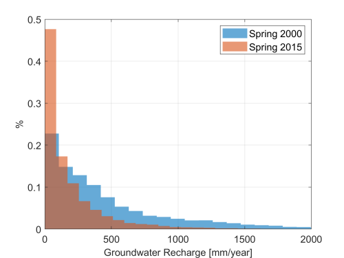
Here we demonstrate vertical travel time through the unsaturated zone for two scenarios:  a typical, average water year (year 2000) and a dry year during the middle of a longer drought (year 2015). The annual recharge rate for these two years are significantly different, with much less recharge in 2015 (dry water year) than in 2000 (average water year).  We note that any other recharge map for the Central Valley may be employed in the same fashion.  Here we use the recharge maps for 2000 and 2015 obtained from C2VSim and plot their respective histograms:

Depth to groundwater

Depth to groundwater is available from two types of sources:

• measured data of depth to water table across a discrete set of wells distributed unevenly across the Central Valley. These data are relatively precise, but they represent only local conditions and are not easily interpolated between measurement locations.
• estimated data from computer simulations of Central Valley groundwater flow during the past 40 to 100 years. Simulations provide spatially continuous maps of water table depth, depicting local variations in water table depth due to local pumping, the presence of rivers and lakes, and also reflecting the heterogeneity in subsurface geologic conditions.  However, water table depth are associated with significant uncertainty.

Here we employ a hybrid approach using both data sources to take advantage of the precision of measured data on one hand, and the continuity of simulated data on the other hand.  The approach preserves the undulating nature of the water table surface, estimated from the simulation model, as much as possible, while forcing the water table surface to coincide with the measured depth to the water table at the exact locations of the measured wells.

The measured data were obtained from the Department of Water Resources.  Simulated water table depth are available from the C2VSim and CVHM models for the Central Valley.  Here, we again use C2VSim results. These data yield the following information, for spring 2000 and for spring 2015:

• Measured data at well locations: Xmeas, Ymeas, Dmeas (x,y coordinates of the measured locations and measured water table depth)
• Simulated data at the finite difference cell or finite element of the simulation grid: Xsim, Ysim, Dsim (x,y coordinates of the simulated water table depth locations, usually one to several points per square mile throughout the Central Valley)

In the following we denote as F(x, y, X, Y, D) an interpolation that uses the data at X,Y locations to interpolate D at the x,y locations.

The steps to condition the simulated data with the measured data are as follows:

1. Obtain "simulated well measurements", Dsim_meas: Extract the simulated depth to the water table by interpolating simulated water table depth to each location at which measurement data are available (well locations):
   Dsim_meas (Xmeas, Ymeas) = F(Xmeas, Ymeas, Xsim, Ysim, Dsim)
   We assume that the high density of grid cells / finite elements yields a negligible error for Dsim_meas.
2. Obtain an "interpolated water table depth based on simulated well measurements", Dsim_interp: Using only the simulated data, Dsim_meas, at the measured well locations, we perform an interpolation of those simulated well measurements, which yields a continuous, interpolated map of an estimated depth to the  (simulated) water table across the entire Central Valley. This interpolated map of the simulated water table depth is different from the simulated map of water table depth, except at the simulated well measurement locations, which are also the locations of real well measurements.  The interpolated water table depth across the finite difference cells/finite elements of the simulation grid, based on simulated well measurements is
   Dsim_interp(Xsim, Ysim) = F(Xsim, Ysim, Xmeas, Ymeas, Dsim_meas)
3. We now consider the difference between the original simulated map of water table depth, Dsim, and the estimated map of simulated water table depth based on simulated well measurement data, Dsim_interp.  This difference represents the exact error introduced by the interpolation method (e.g., kriging) relative to the physically simulated water table depth at locations away from the well locations with (simulated) measurements. The error at any one location will be a function of the density and spatial distribution of the measured data. The estimation error is: 
   Derror(Xsim, Ysim) = Dsim - Dsim_interp
   Note that Derror = 0 at the measured well locations and, hence, simulated well measurement locations.
4. We now repeat the exact same interpolation of step 2, but using the actual measured data instead to obtain an estimated depth of water table at the simulation grid cell locations:
   Dmeas_interp(Xsim, Ysim) = F(Xsim, Ysim, Xmeas, Ymeas, Dmeas)
5. Finally, we obtain a conditionally interpolated depth to groundwater, Dgw, by adding the estimation error computed in step 3 to the interpolated depth to groundwater obtained from measured data:
   Dgw(Xsim, Ysim) =  Dmeas_interp + Derror
   This step preserves, as closely as possible, the undulations in the water table captured by the simulation, here reflected in the magnitude of Derror, while preserving the measured depth to groundwater at the well locations. Derror = 0 at the locations of these wells due to having selected those locations when we obtained Dsim_meas.

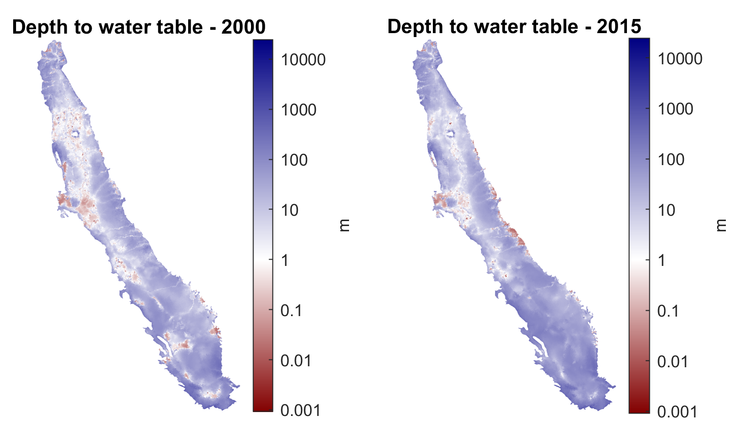
The above algorithm to obtain conditional interpolated water table depth across the (high density) simulation grid yields the following depth to groundwater maps for spring 2000 and 2015 at a one square mile resolution:

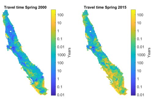
The travel time can now be calculated for given θ values in each of the two example years. For example the travel time distribution for θ=0.05 is