The California Central Valley Groundwater-Surface Water Simulation Model (C2VSim) simulates water movement through the linked land surface, groundwater, and surface water flow systems in California’s Central Valley. Among many other outputs, C2VSim estimates spatially and temporally distributed groundwater recharge. The simulation tool CV-SWAT is a physically based soil-water-crop model, developed mostly to understand the impact of agricultural practices on nitrate and salt leaching. To do so, it also simulates spatio-temporally distributed groundwater recharge.

Within the CV-NPSAT simulation framework, we link these two models  - C2VSIM provides the information on groundwater properties, specified head boundary conditions and flow boundary conditions including the recharge rate across the top of the aquifer to CV-NPSAT;  and CV-SWAT provides the nitrate transport input boundary condition for CV-NPSAT.  We use the CV-SWAT simulated nitrate concentration in combination with C2VSIM estimated recharge.

Note that nitrate concentration ("C") is the mass of nitrate ("M") per unit volume of recharge ("R"):  C = M/R

In locations, where "R" is the same in C2VSIM and in CV-SWAT, the coupling of the two works perfectly.  But - as happens with models - the two rarely are the same. Here then is the dilemma in the coupling of information from C2VSIM (or CVHM or any other flow model) with CV-SWAT for purpose of defining nitrate transport input boundary condition:

• Since nitrate is regulated in drinking water based on its concentration, we want to set the nitrate transport input to the concentration that is provided by CV-SWAT. However, from a nitrate mass balance perspective, where C2VSIM recharge is much larger than CV-SWAT recharge, the same concentration in more recharge means much more mass of nitrate is being leached.  While the opposite is true, where C2VSIM recharge is much smaller than CV-SWAT.
• Alternatively, we could use the mass "M" of nitrate leaching (lb per acre or kg per hectare) obtained from CV-SWAT (M = C * R, all from CV-SAT) and "dissolve" that in the recharge rate provided by C2VSIM.  That would be a mass-conservative coupling, but then the concentration can be very different if CV-SWAT and C2VSIM recharge numbers are very different.

We chose to go with the first approach (use CV-SWAT concentration as nitrate input condition for CV-NPSAT), and instead work on minimizing the differences in recharge obtained from C2VSIM and from CV-SWAT.

How do we minimize these differences?

An important aspect of CV-SWAT is that it operates at a much finer spatial resolution than C2VSIM (or CVHM):  it considers crops and management practices of individual fields and even the different soil types within a field or parcel - which may be as small as a few tens of acres.   In contrast, C2VSIM (or CVHM) lump these differences and estimate recharge at the scale of an individual simulation grid "element" (C2VSIM) or "block" (CVHM), an area that is several hundreds of acres (1 square = 640 acres).  In building CV-NPSAT, we want to take advantage of the more granular information of CV-SWAT, while preserving the overall water mass balance of C2VSIM (or CVHM) either at the groundwater sub-basin scale (more specifically, the 21 water accounting areas in C2VSIM and CVHM) or at the element (block) grid scale (see below).

To explore the differences between the two models we have prepared two GIS applications available at the following links:

• C2VSim Recharge Analysis
• C2VSim CV-SWAT groundwater recharge link

In the following we will provide a description of the GIS layers that are shown in these applications. Both of these tools are based on the earth engine.

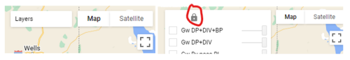
Before delving into the applications it is worth mentioning that earth engine provides a handy feature that can easily be overlooked. At the top right corner there is a layer menu that can be expanded and locked in place with the padlock (red circle), while the sliders can adjust the opacity so that one can easily overlay two or more layers.

C2VSim Recharge Analysis

This application explores the components of C2VSim that are related to groundwater recharge.  C2VSIM considers recharge from five different land use classes:

• native and riparian vegetation (NRV),
• irrigated (non-ponded) agricultural land (NON PONDED),
• wetlands and wildlife refuges (REFUGE),
• rice (RICE), and
• urban areas (URBAN).

C2VSIM further considers three types of groundwater recharge, all three of which may occur in the same grid element or on the corner ("node") of a grid element:

• incidental recharge from the landscape due to precipitation and irrigation being larger than what the soil can hold in the rootzone for plant-soil evapotranspiration (GW DEEP PERCOLATION, "DP");  this is the same conceptual category of recharge considered in CV-SWAT - basically this is the recharge we want to match between CV-SWAT and C2VSIM.
• recharge from canals, ditches, and streams:  C2VSIM calls this "diversion recoverable losses" ("GW Diversion RL" or "DIV"). It is assumed to quickly and directly recharge groundwater and in almost all cases would be water that is low in nitrate concentration (< 2 mg NO3-N/L).  CV-SWAT does not concern itself with this recharge since it is not a groundwater model.
• managed or unmanaged aquifer recharge in floodplains, recharge basins, wetlands etc:  C2VSIM calls this "bypass recoverable losses" ("GW Bypass RL"or "BP").  CV-SWAT also does not concern itself with this. And for purposes of CV-NPSAT, this type of recharge water is also assumed to ahve negligible amounts of nitrate.  

Root Zone (RZ) layers

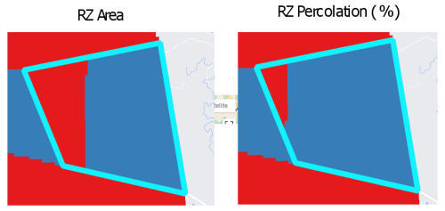
Starting from the bottom of the layer list the RZ Area shows a schematic illustration of the area percentage that each of the five main land use categories take up in each element. In the following figure we show an element that consists of two land use categories i.e. native and riparian vegetation (NRV) and non ponded agriculture (NPA). The RZ Area shows the area percentage but not  where these land uses are located within the element. In a similar manner, the RZ Percolation (%) layer shows the percolation percentage of the NVR and NPA. We can see that although NPA land occupies 60% of the total area the contribution of NPA to the total percolation of the element is about 80%.  

 

The layer RZ Percolation shows the percolation rate per element.

Groundwater (Gw) layers

The layers with GW prefix are related to the three types of groundwater recharge described above: i) Deep percolation (DP), ii) Diversion (DIV) recoverable loss (RL) and iii) By pass (BP) recoverable losses (RL).

The two top layer selections on this map allow the user to see the sum of recharge from DP + DIV and the sum of recharge from DP + DIV + BP

 

C2VSim CV-SWAT groundwater recharge link

This application shows a several layers of groundwater recharge from various models and the inkage results.

LU NASS layers

At the bottom of the layer list we provide two layers that shows the crop categories from the USDA's Crop Land Data for the years 2014 and 2019. Since a legend is not provided it is possible to instead click on the map and the app will display the crop names for these two years at the top left side panel.

CVHM RCH

This is the long-term average groundwater recharge estimated from Central Valley Hydrologic Model (CVHM). The CVHM MOD layer is explained later.

C2VSim II RCH

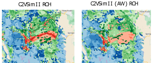
This is the long-term average groundwater recharge estimated from C2VSim. Here we provide two maps: i) the C2VSim II RCH and ii) the C2VSim II (AW) RCH where AW stands for Area Weighted. In C2VSim the diverted water from the streams is distributed over multiple elements. By default, C2VSim distributes the diversion volume equally among elements, regardless of the element size. For example, if the diversion is 100 TAF (thousand acre-feet) and it is distributed to 10 elements, each element receives 10 TAF. This equal spreading results in higher recharge rates where the elements are smaller and lower recharge rates in the larger elements. Alternatively, (for purposes of developing flow boundary conditions for CV-NPSAT), we consider an area weighted (AW) approach.  In the AW approach, the total diversion volume is distributed across the distributed across receiving elements proportional to their size, making the recharge amount (in acre-feet per year) different between elements, but with the recharge rate (in acre-feet/acre per year) being now equal across these elements.

The AW map shows a custom C2VSIM simulation results that distributes DP and BP in an area weighted manner across associated receiving elements, such that the recharge rate is equal across the elements receiving water from a specific diversion. Note that the calibrated C2VSIM version by DWR uses the first approach. The following figure zooms into the Tulare area where the two methods exhibit largest differences in groundwater recharge.

SWAT II

This layer shows the recharge rates based on the CV-SWAT. It does not include the groundwater recharge from diversions or from managed aquifer recharge operations. It is also based on a single year land use map. However the spatial resolution is very detailed.

MOD Layers

The layer list includes a number of MOD layers e.g. CVHM MOD, SVSIM MOD, C2VSim MOD etc. These are the model layers modified based on SWAT crop pattern. Here we briefly describe the methodology we follow for those modifications

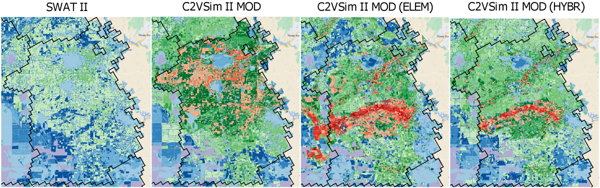
We first began this exercise by preserving the total amount of C2VSIM (or CVHM) recharge at the scale of their 21 water accounting sub-regions (layer with black lines;  also called "Farms" in CVHM). These sub-regions roughly correspond to the Central Valley groundwater sub-basins.  For each of the 21 regions, we compute the total C2VSIM or CVHM recharge, then we distribute that recharge volume across the region proportional to the recharge rates of SWAT II. In other words, we preserve the spatial pattern of recharge obtained from SWAT II, while honoring the total volume of recharge obtained by C2VSIM or CVHM for the water accounting sub-region. The first panel of the figure below shows the recharge rates based on SWAT II for one of the sub-regions. The second panel shows the same recharge pattern scaled so that the total volume of the sub-region is equal to the total volume calculated by C2VSim. This is the layer C2VSim II MOD. It nicely reproduces the very granular SWAT recharge pattern, while being consistent with the overall much higher recharge rates simulated by the C2VSim hydrology. However, in this simulation, the total C2VSIM recharge lumps landscape recharge DP, diversion recoverable losses DIV, and managed aquifer recharge BP all together, then redistributes it across the landscape. This is undesirable, because DIV and BP are actually not associated with carrying nitrate.

In an intermediary next step, we aggregate only to the grid scale rather than the sub-region scale. In other words, we honor the water balance of C2VSIM at the grid element scale.  This is shown in the layer C2VSim MOD (ELEM). The later approach follows precisely the C2VSim hydrology at the grid element scale and it adds the detailed patterns of recharge from CV-SWAT within each element. Artificial patterns that arise from the grid element discretization now become visible.

Finally, we take out the DIV and DP recharge from the landscape recharge.  Within each element we only distribute DP (deep percolation) according to the CV-SWAT recharge pattern.  A grid element's total recharge from canals and ditches (DIV) plus the managed aquifer recharge (BP) is added uniformly to the grid element (and will be accounted for separately in CV-NPSAT's nitrate boundary condition as "clean" recharge) (layer C2VSim MOD (HYBR)).

 

SVSIM and SVSIM MOD

These two layers are analogous to C2VSim and C2VSim II MOD, but using the Sacramento Valley groundwater model.

C2VSim III layers

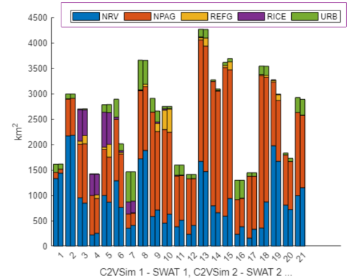
The last two layers show yet another attempt to redistribute SWAT II. The third version builds on top of the C2VSim II MOD (HYBR) approach with additional information from the root zone budget of C2VSim. The major difference in the version C2VSim III MOD DP is that deep percolation is not distributed uniformly across a grid element. Instead it is distributed separately according to it's affiliation with each of the five land use categories in a grid element. The total groundwater recharge volume per subregion is split into Native/Riparian vegetation, Non ponded ag, Refuge, Rice and Urban. This splitting is based on the percentage of root zone percolation (see above). We calculate the cumulative root zone percolation of the 5 categories and split the deep percolation based on the cumulative values. Next we identify which areas are characterized as Urban, Rice etc, in the SWAT layer, which actually maps out each of these land use categories (C2VSIM does not have a map, just land area).  We then redistribute recharge onto the maps of each land use category separately. A very important consideration in this approach is that the two maps should consist of similar acreages per land use category. The following figure shows a comparison between the C2VSim and SWAT areas for each subregion. We can see that there is good agreement between the two models.

 

The last layer C2VSim III MOD is the  C2VSim III MOD DP plus the diversions and bypasses flows.